Dynamic Connectivity¶

Exploring the dynamics of timeseries data with timecorr¶

Written by Jeremy Manning

The timecorr Python toolbox provides tools for computing and exploring the correlational structure of timeseries data. The details of this approach are described in this preprint; some excerpts from the methods of that paper are reproduced below for convenience.

In its most basic usage, the timecorr function provided by the toolbox takes as input a number-of-timepoints (\(T\)) by number-of-features (\(K\)) matrix, and returns as output a \(K \times K \times T\) tensor containing a timeseries of the moment-by-moment correlations reflected in the data. There are two additional special features of the timecorr toolbox that we’ll also explore in this tutorial: dynamic inter-subject functional correlations and high-order dynamic correlations. Before explaining those additional features, we’ll expand on how timecorr estimates dynamic correlations from multi-dimensional timeseries data.

Given a \(T\) by \(K\) matrix of observations, \(\mathbf{X}\), we can compute the (static) Pearson’s correlation between any pair of columns, \(\mathbf{X}(\cdot, i)\) and \(\mathbf{X}(\cdot, j)\) using:

\[\begin{split} \begin{align} \mathrm{corr}(\mathbf{X}(\cdot, i), \mathbf{X}(\cdot, j)) &=\frac{\sum_{t=1}^T \left(\mathbf{X}(t,i) - \bar{\mathbf{X}}(\cdot,i)\right) \left(\mathbf{X}(t, - \bar{\mathbf{X}}(\cdot, j)\right)}{\sqrt{\sum_{t=1}^T \sigma^2_{\mathbf{X}(\cdot, i)} \sigma^2_{\mathbf{X}(\cdot,j)}}},~\mathrm{where}\label{eqn:corr}\\ \bar{\mathbf{X}}(\cdot, k) &= \frac{1}{T}\sum_{t=1}^T \mathbf{X}(t, k),~\mathrm{and}\\ \sigma^2_{\mathbf{X}(\cdot, k)} &= \frac{1}{T}\sum_{t=1}^T \left( \mathbf{X}(t, k) - \bar{\mathbf{X}}(\cdot, k) \right)^2 \end{align} \end{split}\]

We can generalize this formula to compute time-varying correlations by incorporating a kernel function that takes a time \(t\) as input, and returns how much the observed data at each timepoint \(\tau \in \left[ -\infty, \infty \right]\) contributes to the estimated instantaneous correlation at time \(t\).

Given a kernel function \(\kappa_t(\cdot)\) for timepoint \(t\), evaluated at timepoints \(\tau \in \left[ 1, ..., T \right]\), we can update the static correlation formula above to estimate the instantaneous correlation at timepoint \(t\):

\[\begin{split} \begin{align} \mathrm{timecorr}_{\kappa_t}\left(\mathbf{X}(\cdot, i), \mathbf{X}(\cdot, j)\right) &= \frac{\sum_{\tau=1}^T \left( \mathbf{X}(\tau, i) - \widetilde{\mathbf{X}}_{\kappa_t}(\cdot, i) \right) \left( \mathbf{X}(\tau, j) - \widetilde{\mathbf{X}}_{\kappa_t}(\cdot, j)\right)} {\sqrt{\sum_{\tau=1}^T \widetilde{\sigma}_{\kappa_t}^2(\mathbf{X}(\cdot, i)) \widetilde{\sigma}_{\kappa_t}^2(\mathbf{X}(\cdot, j))}},~\mathrm{where}\label{eqn:timecorr}\\ \widetilde{\mathbf{X}}_{\kappa_t}(\cdot, k) &= \sum_{\tau=1}^T \kappa_t(\tau)\mathbf{X}(\tau, k),~\mathrm{and}\\ \widetilde{\sigma}_{\kappa_t}^2(\mathbf{X}(\cdot, k)) &= \sum_{\tau=1}^T \left( \mathbf{X}(\tau, k) - \widetilde{\mathbf{X}}_{\kappa_t}(\cdot, k) \right)^2. \end{align} \end{split}\]

Here \(\mathrm{timecorr}_{\kappa_t}(\mathbf{X}(\cdot, i), \mathbf{X}(\cdot, j))\) reflects the correlation at time \(t\) between columns \(i\) and \(j\) of \(\mathbf{X}\), estimated using the kernel \(\kappa_t\). We evaluate the timecorr equation in turn for each pair of columns in \(\mathbf{X}\) and for kernels centered on each timepoint in the timeseries, respectively, to obtain a \(K \times K \times T\) timeseries of dynamic correlations, \(\mathbf{Y}\).

Dynamic inter-subject functional correlations (dISFC)¶

Given a multi-subject dataset, Simony et al. (2016) define a measure of stimulus-driven inter-regional correlations called inter-subject functional correlation (ISFC). The timecorr toolbox extends this idea to compute a timeseries of ISFC matrices from a multi-subject dataset. (The original ISFC approach computes a static ISFC matrix, although the authors of the original study use a sliding window approach to approximate a timeseries.)

Dynamic high-order functional correlations¶

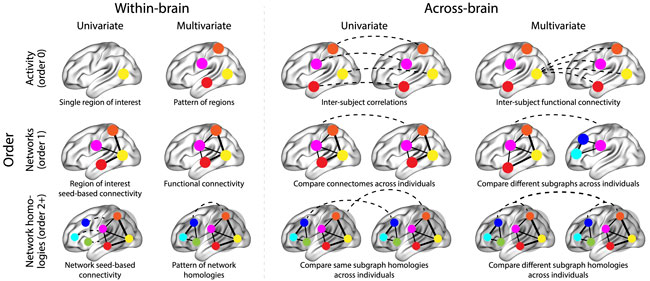
The image below summarizes a variety of neural patterns that one could (in principle) compute or estimate from a neural dataset. Within-brain analyses are carried out within a single brain, whereas across-brain analyses compare neural patterns across two or more individuals’ brains. Univariate analyses characterize the activities of individual units (e.g., nodes, small networks, hierarchies of networks, etc.), whereas multivariate analyses characterize the patterns of activities across units. Order 0 patterns involve individual nodes; order 1 patterns involve node-node interactions; order 2 (and higher) patterns relate to interactions between homologous networks. Each of these patterns may be static (e.g., averaging over time) or dynamic.

500px

Computing high-order functional correlations naively would be computationally intractable for even modest numbers of nodes (brain regions) and orders. This is because the resulting patterns at each timepoint scale exponentially with the order of interactions one attempts to investigate. To make the computations tractable, we use the so-called kernel trick popularized in classification approaches. Rather than carrying out the computations in the “native” feature space (i.e., exponential scaling), we first project the data onto a much lower dimensional space (with \(K\) dimensions), and then we perform the key computations in the low-dimensional space. This enables us to achieve linear scaling with the order of functional correlations, at the expense of precision (since low-dimensional embeddings are lossy). We primarily use two approaches for “embedding” the high-dimensional dynamic correlations in a \(K\)-dimensional space:

400px

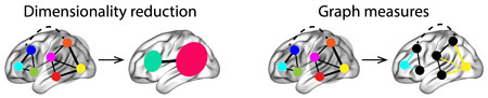
Dimensionality reduction approaches take the \(\mathcal{O}(K^2)\) patterns and embed them in a \(K\)-dimensional space that preserves (to the extent possible) the relations between the patterns at different timepoints. Graph measure approaches forgo attempts to preserve the original activity patterns in favor of instead preserving each node’s changing positions within the broader network (with respect to other nodes).

An overview of the timecorr approach, along with a summary of some of the key findings from this paper may be found in this video (credit: Lucy Owen; recording of a talk she gave at Indiana University).

from IPython.display import YouTubeVideo
YouTubeVideo('y1HYFXVJ5to')

Getting Started¶

Before getting started with this tutorial, we need to make sure you have the necessary software installed and data downloaded.

Software¶

This tutorial requires the following Python packages to be installed. See the Software Installation tutorial for more information.

seaborn
matplotlib
bokeh
holoviews
numpy
pandas
nltools
datalad

Let’s now load the modules we will be using for this tutorial.

import os
from glob import glob as lsdir
import numpy as np
import pandas as pd
from nltools.mask import create_sphere, expand_mask
from nltools.data import Brain_Data, Adjacency
from nilearn.plotting import plot_stat_map

import timecorr as tc
import seaborn as sns
import holoviews as hv
from holoviews import opts, dim

from bokeh.io import curdoc
from bokeh.layouts import layout
from bokeh.models import Slider, Button
from bokeh.embed import file_html
from bokeh.resources import CDN
import panel as pn
import IPython
import datalad.api as dl

import warnings
warnings.simplefilter('ignore')

%matplotlib inline
hv.extension('bokeh')
hv.output(size=200)

Data¶

This tutorial will be using the Sherlock dataset and will require downloading the Average ROI csv files.

We have already extracted the data for you to make this easier and have written out the average activity within each ROI into a separate csv file for each participant. If you would like to get practice doing this yourself, here is the code we used. Note that we are working with the hdf5 files as they load much faster than the nifti images, but either one will work for this example.

for scan in ['Part1', 'Part2']:
    file_list = glob.glob(os.path.join(data_dir, 'fmriprep', '*', 'func', f'*crop*{scan}*hdf5'))
    for f in file_list:
        sub = os.path.basename(f).split('_')[0]
        print(sub)
        data = Brain_Data(f)
        roi = data.extract_roi(mask)
        pd.DataFrame(roi.T).to_csv(os.path.join(os.path.dirname(f), f"{sub}_{scan}_Average_ROI_n50.csv" ), index=False)

You will want to change datadir to wherever you have installed the Sherlock datalad repository. We will initialize a datalad dataset instance and get the files we need for this tutorial. If you’ve already downloaded everything, this cell should execute quickly. See the Download Data Tutorial for more information about how to install and use datalad.

datadir = '/Volumes/Engram/Data/Sherlock'

# If dataset hasn't been installed, clone from GIN repository
if not os.path.exists(datadir):
    dl.clone(source='https://gin.g-node.org/ljchang/Sherlock', path=datadir)

# Initialize dataset
ds = dl.Dataset(datadir)

# Get Cropped & Denoised CSV Files
result = ds.get(lsdir(os.path.join(datadir, 'fmriprep', '*', 'func', f'*Average_ROI*csv')))

A region of interest-based approach to inferring dynamic correlations¶

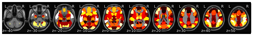
To speed up our computations and make the final results easier to visualize, we’ll use timecorr to estimate connectivity patterns between regions of interest, rather than between the original voxels. Following the Functional Alignment tutorial, we’ll use a 50-ROI mask.

mask = Brain_Data('https://neurovault.org/media/images/8423/k50_2mm.nii.gz')
vectorized_mask = expand_mask(mask)
mask.plot()

rois = pd.read_csv('https://raw.githubusercontent.com/naturalistic-data-analysis/tutorial_development/master/hypertools/rois.csv', header=None, names=['ID', 'Region'])
rois.head()

	ID	Region
0	0	Anterior MPFC
1	1	Fusiform/parahippocampus
2	2	DMPFC
3	3	Sensorimotor/postcentral gyrus
4	4	V1

Next, we’ll extract the mean activation patterns within each ROI.

sub_list = [os.path.basename(x).split('_')[0] for x in lsdir(os.path.join(datadir, 'fmriprep', '*', 'func', '*Part1*csv'))]
sub_list.sort()

sub_timeseries = []
for sub in sub_list:
    sub_timeseries.append(np.array(pd.read_csv(os.path.join(datadir, 'fmriprep', sub, 'func', f'{sub}_Part1_Average_ROI_n50.csv'))))
data = {'part 1': sub_timeseries}

def array2df(x, rois):
    def safequery(i):
        if i in rois['ID'].values:
            try:
                return rois.query(f'ID == {i}')['Region'].values[0]
            except:
                print(f'error processing ID: {i}')
        else:
            return ''
    df = pd.DataFrame(x, columns=[safequery(i) for i in np.arange(x.shape[1])])
    df.drop(labels=[''], inplace=True, axis='columns')
    return df

part1 = [array2df(x, rois) for x in data['part 1']]

#print out a few rows from a sample dataframe
part1[0].head()

	Anterior MPFC	Fusiform/parahippocampus	DMPFC	Sensorimotor/postcentral gyrus	V1	TPJ posterior supra marginal/angular gyrus	PCC/precuneus	Thalamus	SMA	Precentral gyrus	...	A1	Ventral anterior insula	Superior LOC	Cerebellum (crus)	DLPFC	Right IFG VLPFC	Inferior LOC	Right motor	Somatosensory	STS
0	1.755921	5.826709	1.881618	3.776599	8.665937	4.075354	2.421694	2.864211	2.704671	1.684665	...	8.479704	2.271374	4.367660	1.004956	0.914738	3.266528	4.668272	4.707671	-0.345977	0.681969
1	0.215231	3.223925	0.318326	1.034115	6.734484	2.424592	-2.547924	-2.290534	0.777762	-0.346779	...	6.601288	-0.166975	-0.095155	-0.048363	-0.783906	1.443243	1.621159	1.516929	-0.990622	0.175821
2	1.249452	4.600020	1.738919	-0.285278	10.010041	3.080377	-3.444986	-1.887590	-0.490452	1.301151	...	7.870970	1.996753	-0.195372	-1.385071	0.495036	3.470111	4.277213	-0.890185	-2.802245	2.090336
3	-2.558629	0.388236	-0.604157	-2.239837	4.732418	0.037954	-4.747537	0.111611	-1.536647	-0.761406	...	1.653554	-2.125545	-3.647326	-0.437495	-2.373295	-0.043069	0.717843	-2.727891	-1.339336	-0.180019
4	-1.600927	0.792098	-1.058557	-3.124524	4.884841	-0.203100	-4.648347	-2.059925	-2.232909	0.407795	...	1.352045	-1.673176	-4.333806	-2.170690	-1.767852	1.203035	2.995660	-1.785924	-2.892011	-1.251224

5 rows × 41 columns

Generate a dISFC timeseries¶

To generate a timeseries of inter-subject functional correlations, we can use the timecorr function as follows. Note that the batch_extract_roi function defined above drops unlabeled ROIs, so we are left with 41 regions from the original set of 50:

isfc = tc.timecorr(part1, cfun=tc.isfc, combine=tc.corrmean_combine)

There are a few things to note here. The timecorr function takes as input a numpy array, pandas DataFrame, or a mixed list of arrays and DataFrames. By default, timecorr treats each data matrix (i.e., array or DataFrame) independently. For example, calling

tc.timecorr(part1)

returns a list of arrays, each containing a timeseries of correlations for each participant.

The cfun argument specifies which columns (of which matrices) are correlated. By default, cfun is set to tc.wcorr, which computes the dynamic correlations between the features in each column of the data matrices. By setting cfun to tc.isfc, timecorr will compute the dynamic correlations between each column of each participant’s data matrix and the average columns of all other participants’ data matrices.

The combine argument specifies how the result is handled. By default, combine is set to tc.null_combine, which leaves each participants’ timeseries of correlations as separate matrices. When we set combine to tc.corrmean_combine, the resulting timeseries of correlations are averaged together to create a single ISFC timeseries.

Finally, note the dimensions of the result. We input a list of \(T \times K\) matrices, and we received a single \(T \times [(K^2 - K)/2 + K]\) matrix as output. Since each timepoint’s correlation matrix is symmetric, timecorr automatically saves memory by reshaping the upper triangle and diagonal of each timepoint’s \(K \times K\) correlation matrix into a \([(K^2 - K)/2 + K]\)-dimensional vector. We can recover the \(K \times K\) matrices at each timepoint by using the tc.vec2mat function, and we can revert back to the compact form using tc.mat2vec.

print(f'T = {part1[0].shape[0]}')
print(f'K = {part1[0].shape[1]}')
print(f'Shape of output: (T x [(K^2 - K)/2 + K]) = {isfc.shape}')
print(f'Shape of vec2mat(output): (K x K x T) = {tc.vec2mat(isfc).shape}')
print(f'Shape of mat2vec(vec2mat(output)): (T x [(K^2 - K)/2 + K]) = {tc.mat2vec(tc.vec2mat(isfc)).shape}')

T = 946
K = 41
Shape of output: (T x [(K^2 - K)/2 + K]) = (946, 861)
Shape of vec2mat(output): (K x K x T) = (41, 41, 946)
Shape of mat2vec(vec2mat(output)): (T x [(K^2 - K)/2 + K]) = (946, 861)

Visualize the result using chord diagrams¶

We’ll use a chord diagram generated by the Bokeh backend of HoloViews to visualize the brain connectivity patterns. We’ll need to re-format the correlation matrices into DataFrames that describe the set of connections using four columns (there will be a total of \([(K^2 - K)/2]\) rows in this DataFrame:

source: origin of the connection
target: destination of the connection
value: the strength of the connection
sign: whether the connection is positive (+1) or negative (-1)

def mat2chord(vec, t=0, cthresh=0.25):
    def mat2links(x, ids):
        links = []
        for i in range(x.shape[0]):
            for j in range(i):
                links.append({'source': ids[i], 'target': ids[j], 'value': np.abs(x[i, j]), 'sign': np.sign(x[i, j])})
        return pd.DataFrame(links)
    
    links = mat2links(tc.vec2mat(vec)[:, :, t], rois['ID'])
    chord = hv.Chord((links, hv.Dataset(rois, 'ID'))).select(value=(cthresh, None))
    chord.opts(
        opts.Chord(cmap='Category20', edge_cmap='Category20', edge_color=dim('source').str(), labels='Region', node_color=dim('ID').str())
    )
    return chord

Here’s the first correlation matrix:

hmap = mat2chord(isfc, t=0)

# This is to render chord plot in jupyter-book
html_repr = file_html(pn.Column(hmap).get_root(), CDN)
IPython.display.HTML(html_repr)

Bokeh Application

Now let’s create an interactive figure to display the dynamic network patterns, with a slider for controlling the timepoint:

def timecorr_explorer(x, cthresh=0.25):
    hv.output(max_frames=x.shape[0])
    renderer = hv.renderer('bokeh')    
    return hv.HoloMap({t: mat2chord(x, t=t, cthresh=cthresh) for t in range(x.shape[0])}, kdims='Timestep')

For now, we will just plot 100 timepoints to save time generating the plot. Feel free to change this window.

#display 100 timepoints to save time
hmap1 = timecorr_explorer(isfc[100:200, :]);
hmap1

Unfortunately, bokeh plots with interactive widgets are not rendering in jupyter-books yet, so you will only be able to see the interactive plot if you run the notebook locally. We included a gif to visualize these plots on the website.

order1

Second-order and third-order dynamic correlations¶

Computing high-order dynamic correlations¶

Computing high-order dynamic correlations comprises two general steps, which are performed repeatedly in sequence to obtain order \(n+1\) correlations given an order \(n\) timeseries:

Pass the order \(n\) timeseries through timecorr to obtain an order \(n + 1\) timeseries of dynamic correlations between the order \(n\) features.
Embed the order \(n + 1\) features within a \(K\)-dimensional space, yielding a new \(T \times K\) matrix of order \(n + 1\) dynamic correlations.

Temporal blurring¶

The timecorr equation uses a sliding kernel function, centered on each timepoint \(t\) in turn, to estimate stable correlations at each timepoint. More stable estimates may be obtained using wider kernel functions. However, suppose there are rapid changes in the order \(n - 1\) features. The order \(n\) features will somewhat blur those rapid changes. When order \(n + 1\) features are computed from the order \(n\) features, those will be temporally blurred still more. In general, the amount of temporal blurring increases with the order.

To combat temporal blur, we can use a \(\delta\)-function kernel (which has an infinitely narrow width) to compute all of the features up until order \(n - 1\). Then, we can apply a wider kernel (e.g. a Gaussian or Laplace kernel) to the order \(n - 1\) features in order to compute stable order \(n\) features. In this way, the features at every order maintain similar temporal resolution.

Dynamic high-order inter-subject functional correlations¶

Computing (first-order) inter-subject functional correlations entails correlating (at each timepoint) each column of the data matrix from one participant with each column of the average data matrix (taken across all other participants). This highlights stimulus-driven functional correlations that are common across participants, since only stimulus-driven functional correlations would be expected to be similar across different people exposed to a common stimulus.

When we consider high-order functional correlations, we perform this “comparing across participants” step on the order \(n - 1\) features in order to obtain order \(n\) inter-subject functional correlations. This enables us to home in on stimulus-driven order \(n\) patterns that are stable across people.

Eigenvector centrality as a low-dimensional emedding approach¶

Eigenvector centrality is a graph measure that characterizes each node’s degree of connectivity to other connected nodes. We’ll use the rfun argument of the timecorr function to compute the eigenvector centrality of each node at each timepoint reflected in the \(K \times K \times T\) tensor obtained using timecorr. This will yield a \(T \times K\) timeseries of each node’s position in the broader network.

def high_order_timecorr(x, max_order=3, kernel_fun=tc.helpers.gaussian_weights, kernel_params=tc.helpers.gaussian_params):
    
    raw = {0: x}
    smoothed_combined = {0: tc.smooth(tc.mean_combine(raw[0]), kernel_fun=kernel_fun, kernel_params=kernel_params)}
    
    for n in range(max_order):
        if n < max_order - 1:
            raw[n + 1] = tc.timecorr(raw[n], weights_function=tc.eye_weights, weights_params=tc.eye_params, rfun='eigenvector_centrality') #delta function
        smoothed_combined[n + 1] = tc.timecorr(raw[n], weights_function=kernel_fun, weights_params=kernel_params, cfun=tc.isfc)[0]
    
    return smoothed_combined

features = high_order_timecorr(part1)

Let’s create animations of the order 2 and order 3 patterns:

hmap2 = timecorr_explorer(features[2][100:200, :], cthresh=0.1);
hmap2

order2

hmap3 = timecorr_explorer(features[3][100:200, :], cthresh=0.1);
hmap3

order3

What do dynamic high-order functional correlations mean?¶

What does it mean when two brain regions exhibit strong order 2 correlations at a given moment? A high-level way to think about high-order correlations is that they reflect “interactions between interactions between interactions…between features in the original timeseries” (where you say the word “interaction” \(n\) times to describe order \(n\) correlations). In other words, two regions are correlated at order \(n\) if the way they interact with the rest of the brain at order \(n - 1\) is similar.

When different brain regions display high-order correlations, one interpretation is that the networks they are part of are behaving similarly. That could be because they are carrying out similar computations, processing similar information, receiving similar inputs, etc.

Contributions¶

Jeremy Manning developed the tutorial and code. Luke Chang tested and edited code.

Naturalistic Data Analysis